U.S. Economic Outlook in 2025 Q1 and Latin America’s External Financing Conditions

Authors¹:

Christian Alcarraz, FLAR, Bogotá, Colombia. – calcarraz@flar.net
Carlos Giraldo, FLAR, Bogotá, Colombia. – cgiraldo@flar.net
Andrea Villarreal, FLAR, Bogotá, Colombia. – avillarreal@flar.net
Liz Villegas , FLAR, Bogotá, Colombia. – lvillegas@flar.net

¹ The opinions and visions are the responsibility of the authors. They do not necessarily reflect the opinion of FLAR or its administrative bodies.

In the first quarter of 2025, economic conditions in the United States reflect a labor market showing mixed signals, alongside persistent inflationary pressures. This context may limit the Federal Reserve’s (Fed) room to cut its policy rate, suggesting a scenario of higher international interest rates for a prolonged period. For Latin America, this outlook poses an additional challenge by keeping the cost of external financing elevated, particularly for economies with high levels of exposure to external debt.

The Fed has a dual mandate: to promote employment and keep inflation under control, making it essential to analyze both dimensions. The U.S. labor market has shown mixed signals. While the unemployment rate rose slightly to 4.2% and average wage growth slowed to 3.8% in March, job creation significantly exceeded expectations, with 288,000 new jobs generated compared to the 137,000 projected by the consensus.

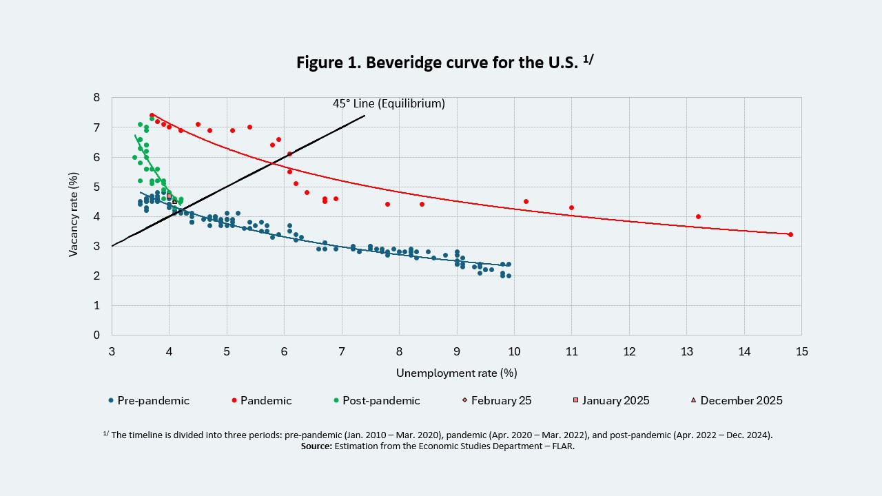
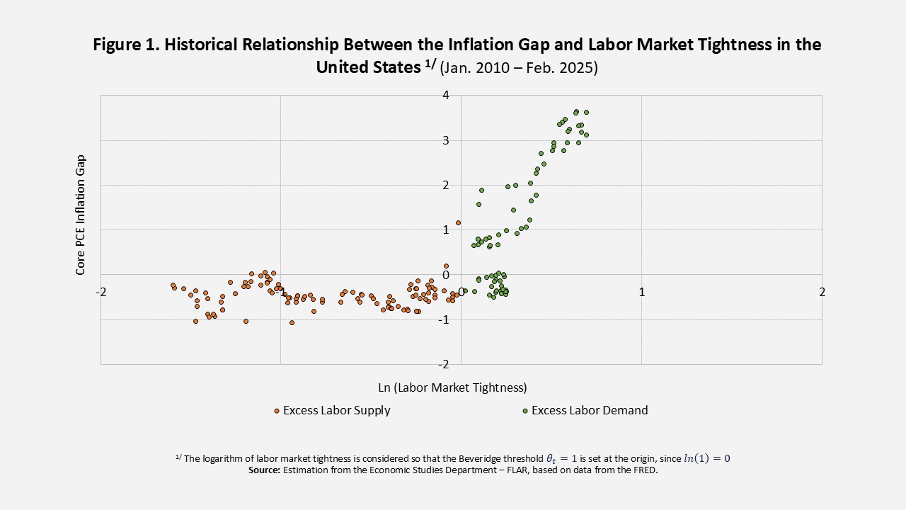
Meanwhile, the Beveridge curve—which illustrates the relationship between the unemployment rate and job vacancy rate—continues to suggest excess labor demand (Figure 1). Although the vacancy rate has been declining, it remains above its pre-pandemic average, helping prevent a significant increase in unemployment in the short term.

Inflation and key indicators remain above the Fed’s target. Both the Consumer Price Index (CPI) and Personal Consumption Expenditures (PCE)—along with their core components—continue to exhibit persistent pressures. The CPI currently stands at 2.8%. Meanwhile, headline PCE has leveled off around 2.5%, while core PCE, which excludes food and energy, has started to pick up, reaching 2.8% as of March 2025.

In addition, most short- and medium-term inflation expectations remain above the Fed’s target. Both household and analyst surveys, as well as market-based indicators, anticipate rising price pressures, partly due to the potential impact of new trade tariffs.

Considering this scenario, in which bringing inflation down has proven more challenging than expected and inflation expectations continue to rise, a key question emerges: Are these dynamics driven by temporary factors, or do they reflect a more structural phenomenon?

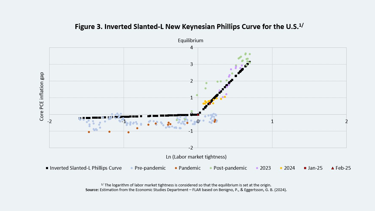
To address this question, we conducted three complementary analytical exercises: (i) A decomposition of the factors behind the core PCE gap, (ii) An estimation of the inverted Phillips curve for the U.S., and (iii) The calculation of instantaneous inflation.

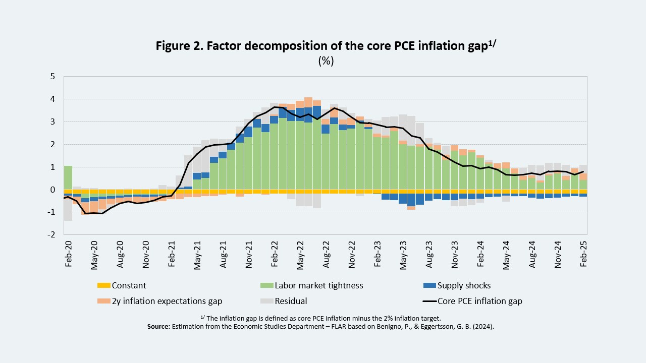
The first exercise, based on the methodology proposed by Beningno and Eggertsson (2024), involves a decomposition of the factors behind the positive gap in core PCE. The results show that the main driver is the vacancy-to-unemployment ratio—a key indicator of labor market tightness—which has played a central role in driving inflationary pressures since 2021. In addition, two-year inflation expectations have contributed to an upward pressure on prices (Figure 2).

This analysis is complemented by the estimation of the inverted Phillips curve for the U.S. (Box 1), which quantifies the relationship between the inflation gap and labor market tightness. The results indicate that the current tightness level stands at 1.10—still too high to close the inflation gap (Figure 3). In fact, the evidence shows that in situations of excess labor demand, the probability of inflation converging to target is just 14%.

Finally, using the methodology proposed by Eeckhout (2023) and the optimal parameter selection criteria from Caicedo, Martínez, and Bonilla (2025)¹, we estimated the instantaneous inflation for core PCE. This indicator assigns greater weight to recent price changes, making it a leading measure of inflation². Recent estimates suggest that short-term inflationary pressures in the U.S. are likely to continue intensifying (Figure 4).

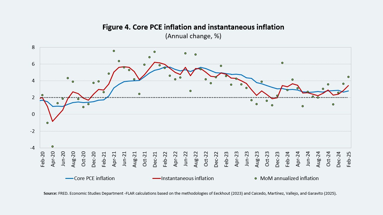
Taken together, the three analyses suggest that inflationary pressures may be less transitory than previously expected, implying that the monetary policy rate could remain unchanged in the short term.

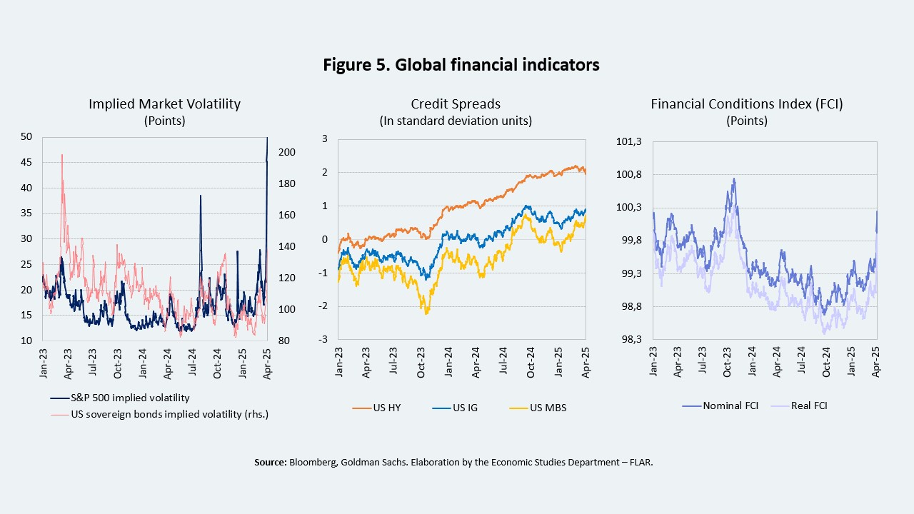
Nonetheless, the global outlook remains exposed to risks with potentially adverse implications for Latin America, particularly stemming from the ongoing trade war. These external shocks could be transmitted to the region through two main channels. First, a prolonged period of high external interest rates would raise external borrowing costs. Second, the recent tightening of global financial conditions—reflected in increased volatility in international markets and wider corporate spreads (Figure 5)—could lead to higher sovereign risk premiums and greater exchange rate volatility across the region.

The recent performance of the U.S. economy points to the persistence of high external financing costs for countries in the region. This underscores the need to maintain economic policy strategies aimed at strengthening resilience in the face of heightened external uncertainty.

¹ We incorporated the methodology presented in the January 2025 Monetary Policy Report by the Banco de la República of Colombia. Using this approach, we optimized the kernel smoothing parameter proposed by Eeckhout (2023) based on the following criteria: (i) maximizing the ratio of inflation explained to the volatility of instantaneous inflation, and (ii) maximizing the ratio of inflation explained to the root mean squared error between instantaneous and observed inflation.

² This methodology gives greater weight to the most recent monthly inflation data to correct the bias in traditional year-over-year inflation calculations, which assign an equal weight to each of the past 12 months.

Box 1. Estimating the Inverted-L Phillips Curve for the United States

The methodology proposed by Beningno and Eggertsson (2024) enables the estimation of the Inverted-L Shaped New Keynesian Phillips Curve for the U.S. —hereafter referred to as the INV-L¹, Curve—as an alternative to the standard New Keynesian Phillips Curve.

The INV-L Curve introduces nonlinearity by estimating two distinct slopes. Inflation’s responsiveness to labor market conditions becomes significantly sharper once a critical threshold of labor market tightness—commonly referred to as the Beveridge threshold—is exceeded. In this regime, characterized by acute labor market tightness, the labor market becomes excessively constrained, amplifying inflationary pressures.

The notion of a nonlinear relationship between inflation and unemployment traces back to Phillips’ (1958) seminal work, which suggested that wage inflation \( \left( \pi_t^w \right) \) is convexly related to the unemployment rate \( \left( u_t \right) \):

\( \pi_t^w = a + b \left( \frac{1}{u_t} \right)^c \)

Where \(a\), \(b\) and \(c\) are parameters to be estimated. Phillips argued that the relationship between unemployment and inflation is inherently nonlinear, driven by asymmetries in wage dynamics. When unemployment is low, labor shortages exert upward pressure on wages; however, when unemployment is high, nominal rigidities prevent wages from falling at the same pace. As a result, the relationship between employment and inflation is neither symmetric nor linear.

The current relationship between the unemployment rate \( \left( u_t \right) \) and job vacancies \( \left( v_t \right) \) is summarized by the Beveridge Curve. To construct a more concise measure of labor market conditions, these two variables are combined into an index known as “labor market tightness”.

This indicator is defined as \( \theta_t = \frac{v_t}{u_t} \) and captures the number of job vacancies per unemployed individual. When \( \theta_t > 1 \) vacancies outnumber unemployed workers, indicating excess labor demand. Conversely, when \( \theta_t < 1 \) unemployment exceeds the number of available job openings, reflecting excess labor supply. A value of \( \theta_t = 1 \) suggests labor market equilibrium, corresponding to a point on the 45-degree line of the Beveridge Curve.

Recent academic² contributions concur that labor market tightness offers a more precise characterization of labor market slack than the unemployment rate considered in isolation³. Beningno and Eggertsson (2024) also attribute part of the post-pandemic “inflation surprise” to the failure of conventional models to account for the nonlinear sensitivity of inflation to labor market conditions. For instance, Hazell, Herreño, Nakamura, and Steinsson (2022), using a multi-regional model for the United States, estimate that a one-percentage-point decline in the unemployment rate leads to a 0.34% increase in inflation.

When examining the historical relationship between the inflation gap⁴ and labor market tightness, the evidence reveals a pronounced asymmetry. Under conditions of excess labor demand \( \left( \theta > 1 \right) \), inflation exhibits substantially greater sensitivity to labor market pressures than in periods of slack. This nonlinearity provides a rationale for estimating an inverted-L shaped Phillips Curve, characterized by two distinct slopes depending on the degree of labor market tightness.

Methodology

In addition to labor market tightness as the core explanatory variable, we include a set of control variables to improve the identification of the inverted-L Phillips Curve (INV-L). The model is estimated using Ordinary Least Squares (OLS):

\( \tilde{\pi}_t = \beta_c + (\beta_\theta + \beta_{\theta_d} D_t) \ln(\theta_t) + (\beta_v + \beta_{v_d} D_t) v_t + \beta_{\tilde{\pi}} \tilde{\pi}^e_t + \epsilon_t \)

\(
\epsilon_t \sim iid\ \mathcal{N}(0, \sigma^2)
\)

Where \( \varepsilon_t \) denotes the Gaussian error term, assumed to be independently and identically distributed with mean zero and constant variance \( \sigma^2 \), \( \tilde{\pi}_t \) refers to the inflation gap, defined as the deviation of year-over-year core PCE inflation from the 2% target, \( {D}_t \) is a dummy variable equal to 1 under conditions of excess labor demand (\( \theta_t > 1 \)) and 0 otherwise. The variable \( \ln(\theta_t) \) aptures the logarithm of labor market tightness, \( v_t \) accounts for supply shocks, and \( \tilde{\pi}_t^e \) represents the two-year ahead inflation expectations gap.

Under this specification, the asymmetric effect of labor market tightness on inflation is explicitly incorporated. The inclusion of the dummy variable \( D_t \) in the slope coefficients allows for the identification of nonlinearity—specifically, the presence of distinct marginal effects—within the structure of the inverted-L Phillips Curve.

\(\frac{\partial \mathbb{E}(\tilde{\pi}_t)}{\partial \ln(\theta_t)} = \beta_{\theta} + \beta_{\theta_d} D_t\)

Therefore, the slope of the Phillips Curve will be conditional on labor market conditions:

\(
\frac{\partial \mathbb{E}(\tilde{\pi}_t)}{\partial \ln(\theta_t)} =
\begin{cases}
\beta_\theta + \beta_{\theta_d}, & \text{si } D_t = 1 \ (\text{Excess Labor Demand}) \\
\beta_\theta, & \text{si } D_t = 0 \ (\text{Excess Labor Supply})
\end{cases}
\)

If \( \beta_{\theta_d} > 0 \), the inflation gap becomes more responsive to labor market tightness under conditions of excess labor demand. In other words, the slope of the Phillips Curve increases when the labor market operates above the Beveridge equilibrium. The statistical significance of this coefficient would provide empirical support for the nonlinearity hypothesis.

Given that supply shocks \( v_t \) are not directly observable, we apply Principal Component Analysis (PCA) to extract a common factor from three variables: (i) The gap between headline and core CPI inflation; (ii) The gap between headline and core PCE inflation; and (iii) The difference between the implicit deflators of imports and GDP.

Data

In Beningno and Eggertsson (2024), the inverted-L Phillips Curve is estimated using quarterly data. However, to capture the inflation dynamics with greater granularity, this analysis employs monthly data spanning from January 2010 to February 2025. This modification introduces a methodological challenge, as the implicit deflators for imports and GDP are available only at quarterly frequency.

To address this limitation, the temporal disaggregation procedure proposed by Chow and Lin (1971) is employed. This method enables the interpolation of low-frequency series into higher-frequency data while preserving aggregate consistency with the original series⁵.

After constructing the series at a monthly frequency, supply shocks are identified through the first principal component extracted from the set of price differentials. This component accounts for 94% of the total variance across the variables, making it a strong summary measure of cost-push shocks that affect inflation dynamics.

Results

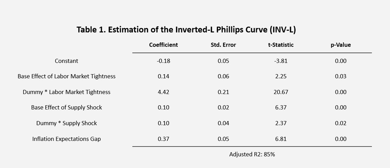
Table 1 presents the regression results. The nonlinearity of the INV-L Phillips Curve—captured by the coefficient associated with the dummy variable for excess labor demand—is statistically significant at the 1% level, with an estimated value of 4.42%, the highest among all explanatory variables.

In periods of excess labor demand, a 1% increase in labor market tightness leads to a 4.56% rise in the inflation gap (elastic segment). In contrast, under excess labor supply (inelastic segment), the same increase in tightness results in only a 0.14% rise in the inflation gap.

Supply shocks are amplified by an additional 0.10% when the labor market operates above the Beveridge equilibrium, relative to periods of slack. This differential effect is also statistically significant at the 1% level.

Furthermore, a 1% increase in the two-year inflation expectations gap is associated with a 0.37% increase in the current inflation gap, underscoring the stabilizing role of well-anchored expectations.

Overall, the model accounts for 85% of the variation in the U.S. inflation gap.

¹ Methodology presented at the 2024 Jackson Hole Global Monetary Policy Symposium.

² Barnichon y Shapiro (2022); Furman y Powell (2021); Domash y Summers (2022).

³ Beningno and Eggertsson (2024) argue that one of the factors contributing to the delayed onset of the Federal Reserve’s policy rate normalization cycle—despite core PCE inflation exceeding the target—was the reliance on traditional labor market indicators, such as the unemployment rate, which remained above its pre-pandemic average of 5.1% (2013–2019)

⁴ Defined as core PCE inflation minus the 2% target.

⁵ The estimation relies on auxiliary indicators: the import price index is used as a proxy for the import deflator, and the consumer price index (CPI) serves as a proxy for the GDP deflator.

References

Barnichon, R., & Shapiro, A. H. (2022). What’s the best measure of economic slack? FRBSF Economic Letter, 2022-04.

Benigno, P., & Eggertsson, G. B. (2024). The Slanted-L Phillips Curve (NBER Working Paper No. 32172). National Bureau of Economic Research. https://doi.org/10.3386/w32172

Chow, G. C., & Lin, A.-L. (1971). Best linear unbiased interpolation, distribution, and extrapolation of time series by related series. The Review of Economics and Statistics, 53(4), 372–375. https://doi.org/10.2307/1928739

Domash, A., & Summers, L. H. (2022). How tight are U.S. labor markets? (NBER Working Paper No. 29739). National Bureau of Economic Research.

Eeckhout, J. (n.d.). Instantaneous Inflation. SSRN. https://ssrn.com/abstract=4554153 or http://dx.doi.org/10.2139/ssrn.4554153

Furman, J., & Powell III, W. (2021). What’s the best measure of labor market tightness? Peterson Institute for International Economics. November 22, 2021.

Hazell, J., Herreño, J., Nakamura, E., & Steinsson, J. (2022). The slope of the Phillips curve: Evidence from U.S. The Quarterly Journal of Economics, 137(3), 1299–1344.

Martínez-Rivera, W., Caicedo-García, E., & Bonilla-Pérez, J. (2025). Instantaneous inflation as a predictor of inflation. Borradores de Economía, 1296, Banco de la República de Colombia.

Phillips, A. W. (1958). The relation between unemployment and the rate of change of money wage rates in the United Kingdom, 1861–1957. Economica, 25(100), 283–299.