Latin America: Macro-financial stability and emerging risks in an uncertain global environment

Authors¹:

Christian Alcarraz, FLAR, Bogotá, Colombia. – calcarraz@flar.net
Carlos Giraldo, FLAR, Bogotá, Colombia. – cgiraldo@flar.net
Andrea Villarreal, FLAR, Bogotá, Colombia. – avillarreal@flar.net
Liz Villegas , FLAR, Bogotá, Colombia. – lvillegas@flar.net

¹ The opinions and visions are the responsibility of the authors. They do not necessarily reflect the opinion of FLAR or its administrative bodies.

In the early months of the year, most economies in the region have shown resilience despite a highly uncertain international environment, characterized by falling commodity prices and rising geopolitical and trade risks. Several economies have experienced a slowdown in real GDP growth and a continuation of the disinflation process, with significant differences across countries. In this context, external financing flows to the region have remained stable.
Looking ahead, countries face different economic risks shaped by a highly uncertain global environment and by their varying capacities for monetary and fiscal policy responses.

Recent External Shocks: Uncertainty, Commodity Prices, and Financing Flows

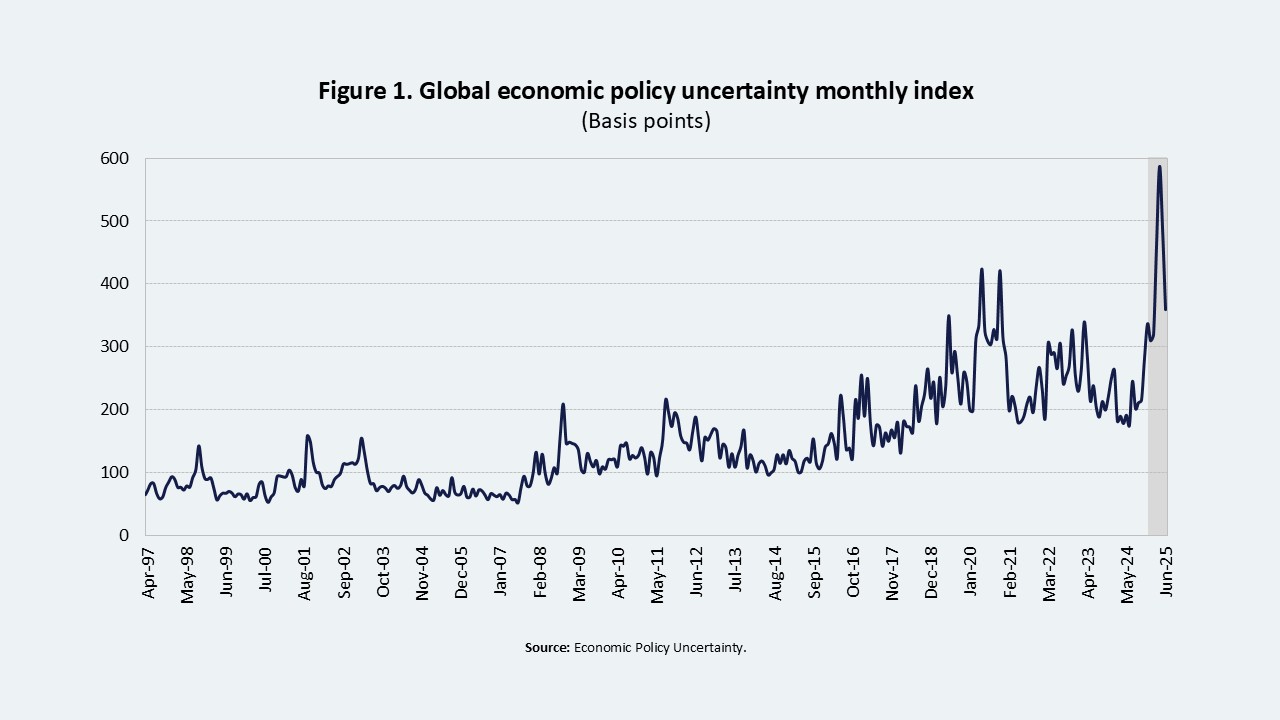
Global economic policy uncertainty has risen to historical levels due to increasing trade tensions (Figure 1). Although the peak in uncertainty was recorded following the announcement of broad-based tariff measures by the administration of Donald Trump (Liberation Day), its subsequent decline has been slow, remaining at elevated levels compared with 2024.

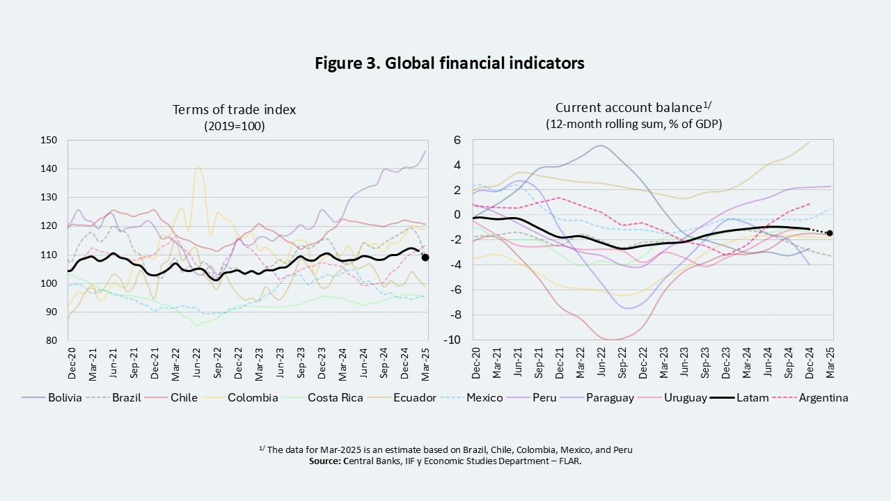
Export prices for the region’s main commodities have declined, except for copper (Figure 2). Its increase could be explained by the U.S. government’s tariff announcements, which may have led to an anticipation of future costs being reflected in current prices, or to a risk premium arising from uncertainty over their implementation.

As a result, the terms of trade of most Latin American countries deteriorated, putting upward pressure on the current account deficit of many commodity-exporting countries during the early months of the year (Figure 3).

Given the prevailing global conditions, preliminary balance of payments data for the first quarter of 2025 suggest that capital flows to Latin America have remained relatively stable and may even have increased as a share of GDP in several economies.

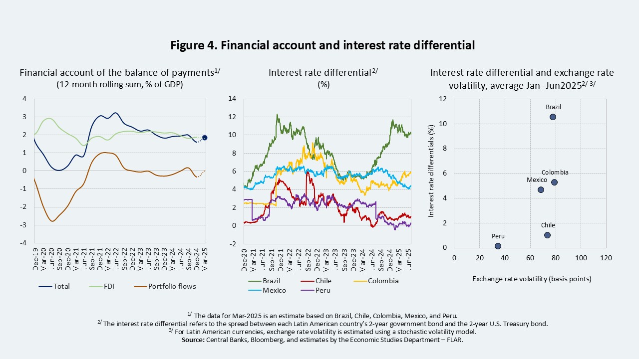
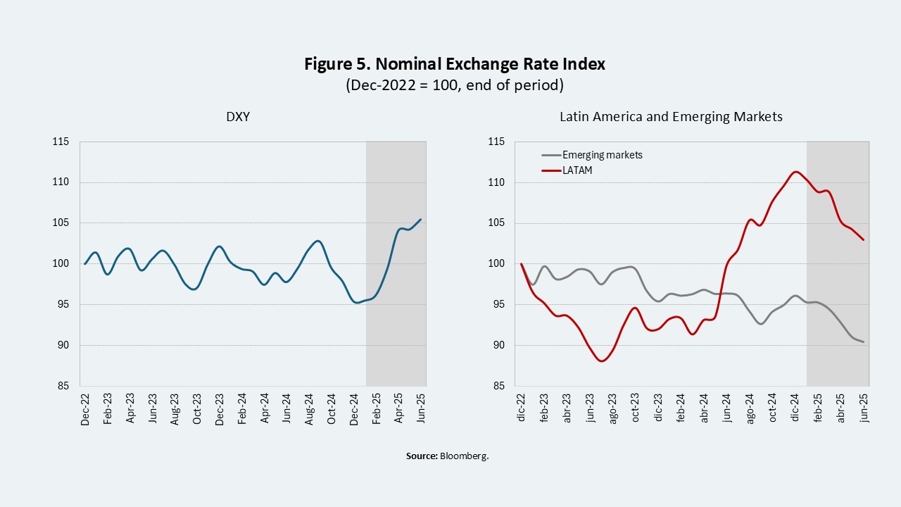
Capital inflows have been predominantly driven by portfolio flows. On the one hand, this may reflect the fact that the interest rate differential relative to dollar,. partly because interest rate differentials relative to dollar-denominated investments remains attractive for carry trade operations, particularly in countries such as Brazil and Colombia (Figure 4). At the same time, the United States has become the epicenter of global uncertainty—due to the trade war and widening fiscal imbalances—weakening the dollar and encouraging investors to diversify into emerging markets, including those in Latin America. This has contributed to the appreciation of most regional currencies (Figure 5).

Growth shaped by external and domestic factors, a gradual disinflation path, and heterogeneous monetary policy responses

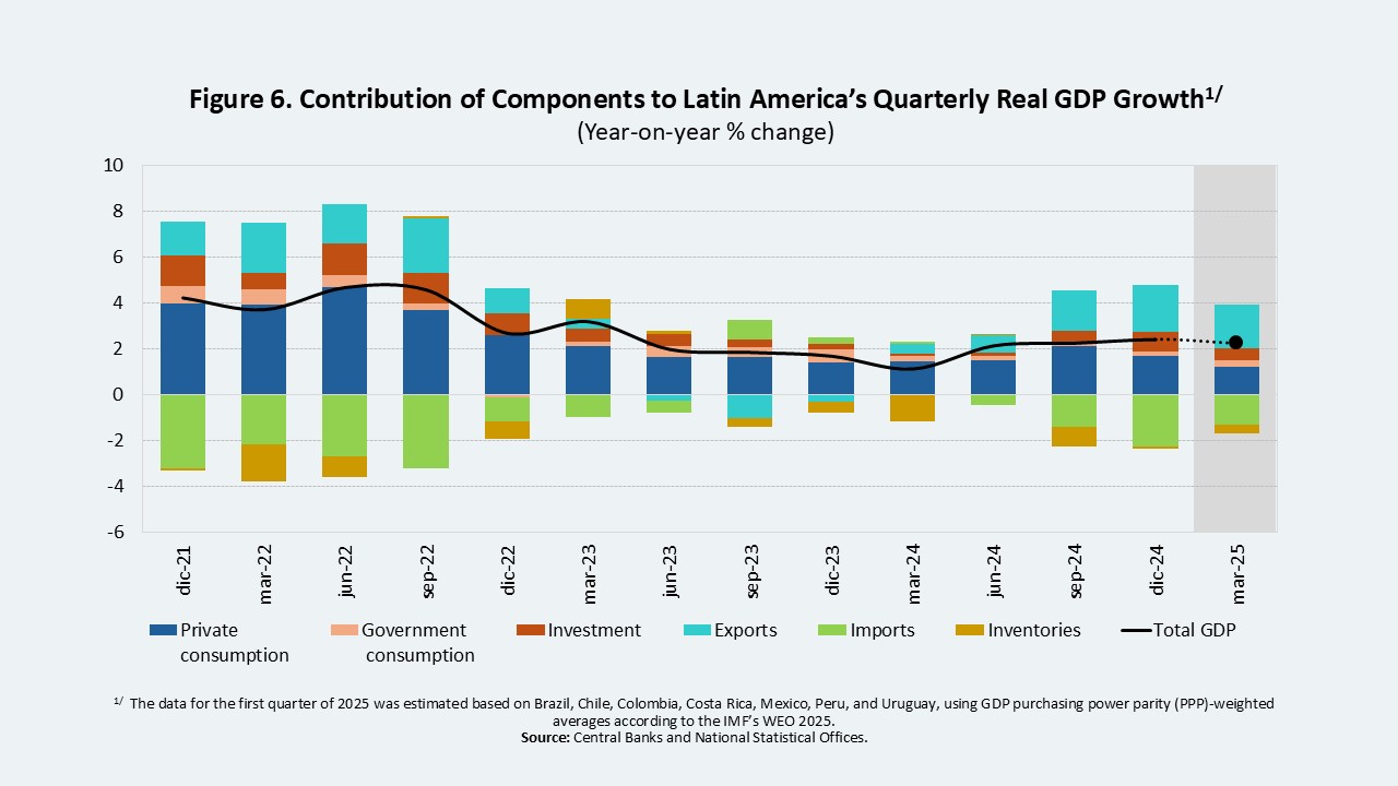
Preliminary real sector data point to lower GDP growth compared with the end of last year for most countries. This has been the result of both external and domestic factors (Figure 6). Export volumes have declined along with weaker external demand and deterioration in terms of trade, while household consumption and private investment have been affected by country-specific factors. These include domestic economic or political uncertainty, low consumer and investor confidence, high household debt, weaker public investment, and elevated interest rates.

In this context, both headline and core inflation have gradually declined in most countries (Figure 7), with the exception of economies such as Bolivia, and to a lesser extent Mexico and Brazil. Meanwhile, monetary policy decisions have been heterogeneous among central banks. While Brazil and Uruguay have continued to raise their policy rates, others such as Chile, Costa Rica, and Peru have chosen to keep theirs unchanged.

High public debt levels and pressure on fiscal balances

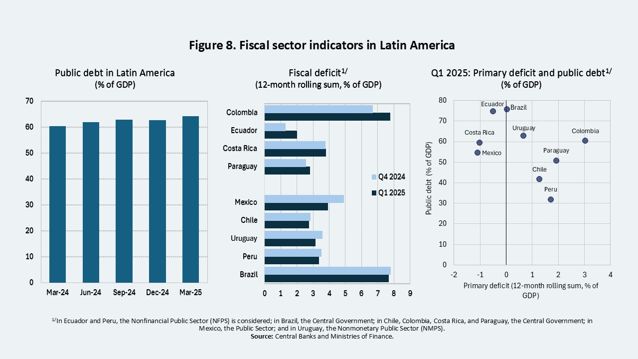
Fiscal conditions are heterogeneous across countries in the region, but concerns persist in several economies due to high and rising public debt levels as a share of GDP (Figure 8). Fiscal deficits are not low enough to stabilize or reduce this ratio. This dynamic reflects both higher primary spending and increased interest payments, the magnitude of which varies by country.

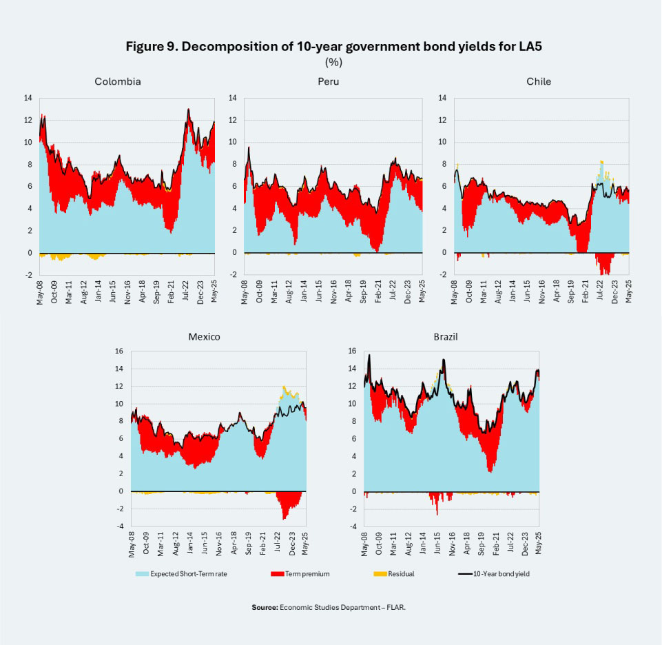
Given the relevance of sovereign financing costs and their impact on the fiscal trajectory, we assessed their structure for five regional economies based on public debt market information across the yield curve. For this purpose, we apply the ACM model (Adrian, Crump, & Moench, 2013), which decomposes long-term interest rates into two components: (i) the expected average of the short-term rate and (ii) the term premium. The first component reflects the expected path of short-term rates, and the second incorporates various risk factors, such as the fiscal deficit, the U.S. term premium, and exchange rate volatility (see Methodological Box).

The results indicate that the term premium has played an important role in long-term rates in countries such as Colombia, Peru, and Chile, and to a lesser extent in Mexico and Brazil (Figure 9). In the latter countries, short-term rates account for most of the behavior of long-term rates.

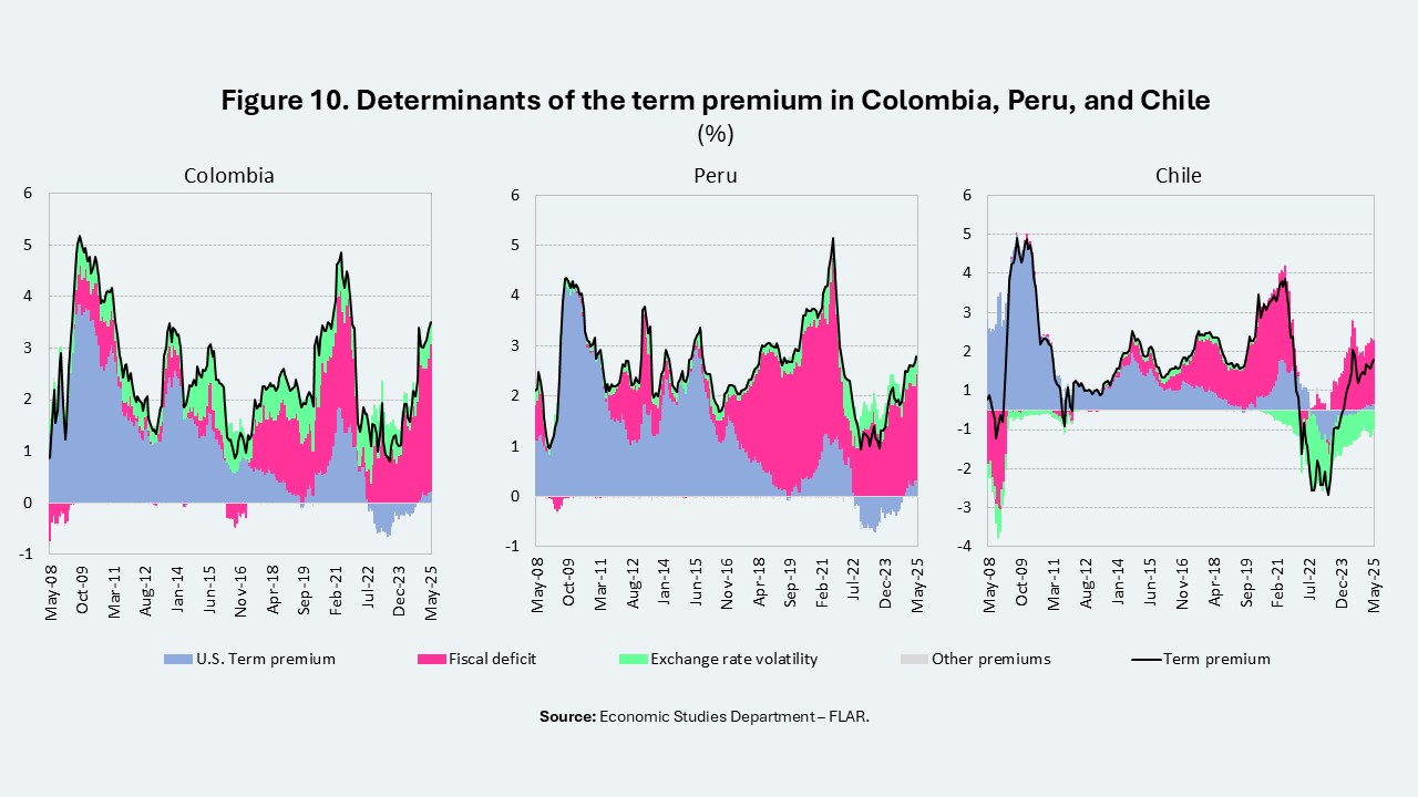
In addition, we estimated the determinants of the term premium for Colombia, Peru, and Chile (see Methodological Box). The results show that the fiscal deficit is the factor that most influences its evolution, particularly in the case of Colombia (Figure 10).

Short-term outlook and risks

For the remainder of the year, Latin America is expected to continue facing a challenging external and domestic environment, consistent with the trends observed so far.

On the external front, GDP growth in the United States and China is expected to be weaker than projected at the beginning of the year. Furthermore, inflation in the United States is expected to remain persistent, in contrast to the Euro Area and China, where weak domestic demand has contributed to its moderation. In the case of the United States, inflation expectations remain above the Federal Reserve’s target.

Given this scenario, the Fed is expected to maintain its current policy rate. This would imply that external financing costs would remain elevated for Latin America (see FlarBlog: “U.S. Economic Outlook in 2025 Q1 and Latin America’s External Financing Conditions”).

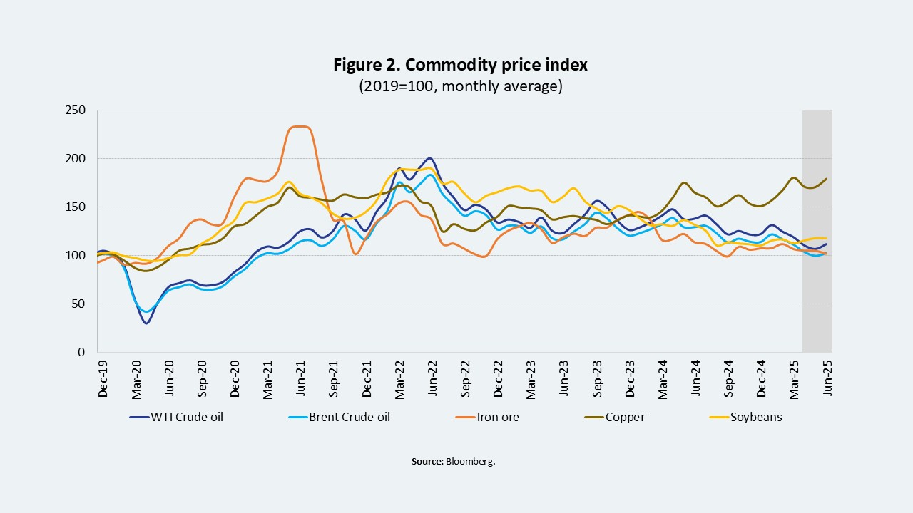
A broad-based decline in commodity prices relevant to the region’s exporters is also projected. This reflects weak global demand and, in some cases, increases in supply (e.g., oil and soybeans).

In addition to the weaker external dynamics, factors related to domestic demand are expected to contribute to slower regional growth. Aggregate demand will remain weak reflecting the elements discussed above, which will continue to constrain both consumption and private investment. In this context, the region—excluding Argentina—is projected to grow by 1.6% 2025, which is below the 2.4% recorded in 2024. However, including Argentina, regional growth would reach 2.0%.

From a fiscal perspective, the region’s aggregate deficit is expected to remain around 6% of GDP. Public debt is projected to reach 62.8% of GDP in 2025, which is above the 60% observed the previous year.

Finally, several short-term risks have been identified, notably: (i) further fiscal deterioration in some countries, with potential implications for macroeconomic stability, (ii) external shocks arising from an escalation of geopolitical and trade tensions, and (iii) a sharper slowdown in external demand, particularly from China.

Methodological Box: Term Structure of Interest Rates and Determinants of the Term Premium in the LA5 Economies

The structure of the yield curve provides key information for central banks. As noted by Ceballos et al. (2015), conventional monetary policy affects the yield curve and, in turn, the financing and spending decisions of households, firms, and the government. In this context, the Expectations Hypothesis (EH), originally formulated by Lutz (1940), argues that long-term interest rates reflect the average of current and expected future short-term rates.

The EH assumes that agents form rational expectations about interest rates without systematic errors (Muth, 1961; Cook and Hahn, 1990). Under this framework, long-term rates should equal the expected average of short-term rates, while forward rates would be unbiased predictors. However, empirical evidence shows that this simple version of the hypothesis does not fully account for the dynamics of long-term rates. This has led to the incorporation of a time-varying term premium (Fama and Bliss, 1987; Campbell and Shiller, 1991).

The term premium represents the compensation investors require for holding long-term bonds instead of rolling over a series of short-term instruments. It also captures duration risk and other macro-financial risks. Consequently, decomposing long-term rates into expected short-term rates and the term premium and identifying the determinants of the latter is crucial for assessing how much of long-term rates reflects monetary policy expectations versus risk perceptions.

Because neither expected short-term rates nor the term premium are directly observable, they must be estimated through models. Among the most widely used are affine term structure models calibrated to the yield curve. The Adrian, Crump, and Moench (2013, hereafter ACM model) framework provides an efficient estimation method based on linear regressions. Its simplicity, combined with results comparable to more complex approaches, has fostered its widespread adoption. In fact, the Federal Reserve Bank of New York regularly publishes estimates of the U.S. term premium using this methodology, which are frequently cited in academic research and the financial press.

An alternative approach is that of Kim and Wright (2005), which incorporates survey-based expectations of three-month Treasury bill yields to estimate expected short-term rates, rather than deriving them solely from the yield curve as in the ACM model. However, due to the lack of consistent historical survey data, this study applies the ACM methodology to five economies in the region: Brazil, Chile, Colombia, Mexico and Peru.

Adrian, Crump, and Moench (ACM) Model

To estimate term premium from the observed market yield curve, the following steps are undertaken.

Sovereign Yield Curve

Consider a yield curve that contains equidistant rates across \(N\) maturities. In practice, however, governments typically issue a smaller number of instruments than the total number of such points \(\)\left( M < N \right)[/latex]. As a result, [latex]N[/latex] points must be interpolated from the M market-observed yields. For this purpose, a four-factor parametric model is employed, following the methodology proposed by Svensson (1995).

\( y_t^{(n)} = \alpha_0 + \alpha_1 \left[ \frac{1 – e^{-\left( \frac{n}{\lambda_1} \right)}}{\frac{n}{\lambda_1}} \right] + \alpha_2 \left[ \frac{1 – e^{-\left( \frac{n}{\lambda_1} \right)} – e^{-\left( \frac{n}{\bar{\lambda}_1} \right)}}{\frac{n}{\lambda_1}} \right] + \alpha_3 \left[ \frac{1 – e^{-\left( \frac{n}{\lambda_2} \right)} – e^{-\left( \frac{n}{\bar{\lambda}_2} \right)}}{\frac{n}{\lambda_2}} \right] + \eta_t^{(n)} \)

\( n = n_1, n_2, n_3, \ldots, n_M \)

Where \(y_t^{(n)}\) denotes the spot rate observed at time \(t\) with maturity \(n\) periods \(\)\left( 0 < t < n \right)[/latex]. The coefficients have the following interpretation (Svensson, 1995; Diebold and Li, 2006):

\(\alpha_0\): Level of the yield curve, associated with the long-term component of interest rates. In other words, it reflects the level to which the yield curve converges as \(n \to \infty\)
\(\alpha_1\): Slope factor, capturing the sensitivity of yields to short-term movements. It primarily affects the short end of the maturity spectrum.
\(\alpha_2\): Curvature factor (first curvature), associated with the medium-term component. It allows for an adjustment of the convexity of the yield curve at intermediate maturities.
\(\alpha_3\): Second curvature factor, associated with an additional curvature component. It allows for further adjustments to the convexity of the yield curve at very short or very long maturities, providing greater flexibility to capture complex dynamics in specific segments of the curve.
\(\lambda_1\): Decay parameter of the first curvature, governing the speed at which the influence of the first curvature factor declines across maturities.
\(\lambda_2\): Decay parameter of the second curvature, governing the speed at which the influence of the second curvature factor diminishes across maturities.

Finally, \(\eta_t^{(\tau)}\) denotes the model error.

Given the nonlinear specification of the model, Nonlinear Least Squares (NLS) is applied in each period \(t\) to estimate the parameters. Based on these estimates, \(N\) yields are interpolated at equidistant maturities \(n = n_1, n_2, n_3, \ldots, n_N\), to obtain a continuous, smooth, and internally consistent representation of the yield curve that facilitates the recursive valuation of sovereign instruments.

Bond Valuation under No-Arbitrage

In the interest rate modeling literature, it is common to assume a no-arbitrage condition under which financial instruments with identical risk characteristics must have the same price. This principle imposes restrictions on the co-movement of yields across maturities and ensures the internal consistency of market prices.

Gaussian affine term structure models assume that yields depend linearly on a set of risk factors (hence the term “affine”), while “Gaussian” refers to the assumption that these factors follow a normal distribution (Dai and Singleton, 2000; Duffee, 2002; Cochrane and Piazzesi, 2005; Joslin et al., 2011; Adrian et al., 2013). Building on this strand of the literature, the following Gaussian affine term structure specification is employed.

Let \(X_t\) be a \(k\) -dimensional vector of risk factors or state variables, whose dynamics under the physical measure \((P)\) are described by a Gaussian VAR(1) process.

\( X_{t+1} = \mu + \Phi X_t + v_{t+1} \)

\( v_{t+1} \sim iid\, N(0, \Sigma) \)

Where the underlying risk factors of the yield curve, with \(k = 3\), are identified using Principal Component Analysis (PCA) and are commonly referred to as level, slope, and curvature (Litterman and Scheinkman, 1991). The level factor represents the average of yields across maturities, the slope factor captures the spread between long- and short-term segments, and the curvature factor reflects movements in the intermediate maturities of the yield curve (Diebold et al., 2004). Other studies extend this specification by incorporating macroeconomic variables as additional risk factors, including Ang and Piazzesi (2003), Crump et al. (2018), Gurkaynak and Wright (2012), and Wright (2011).

Under the no-arbitrage assumption (Dybvig and Ross, 1987), there exists a Stochastic Discount Factor \(M_{t+1}\) (also known as the pricing kernel), which allows the price \(t\) of a zero-coupon bond maturing in \(P_t^{(n)}\) periods to be determined at time \(n\). This factor ensures that model-implied prices are consistent with those observed in the market, thereby ruling out arbitrage opportunities.

\( P_t^{(n)} = E_t \left[ M_{t+1} P_{t+1}^{(n-1)} \right] \)

\( n = n_1, n_2, n_3, \ldots, n_N \)

The stochastic discount factor \(M_{t+1}\) is specified as an exponential-affine function of the risk factors.

\( M_{t+1} = e^{\left( -r_t – \frac{1}{2} \lambda_t’ \lambda_t – \lambda_t’ \Sigma^{-\frac{1}{2}} v_{t+1} \right)} \)

Where \(r_t\) denotes the short-term interest rate (or risk-free rate) associated with the shortest maturity available, defined as \(r_t = \ln \left( P_t^{(1)} \right)\). This rate is affine, or linear, in the risk factors, in line with structural term structure models such as Vasicek (1977).

\( r_t = \delta_0 + \delta_1′ X_t \)

Where \(\delta_0\) and \(\delta_1’\) represent the sensitivity vectors.

Furthermore, following Duffee (2002), the market price of risk \((\lambda_t)\) is defined as:

\( \lambda_t = \Sigma^{-\frac{1}{2}} \left( \lambda_0 + \lambda_1 X_t \right) \)

Where \(\lambda_0\) and \(\lambda_1\) represent the sensitivity vectors.

Once bond prices are obtained, the corresponding yields \(y_t^{(n)}\) can be derived through the following relationship:

\( y_t^{(n)} = -\frac{1}{n} \ln\left(P_t^{(n)}\right) \)

The one-period excess return on a bond with maturity \(n\) is defined as:

\( rx_{t+1}^{(n-1)} = \ln\left(P_{t+1}^{(n-1)}\right) – \ln\left(P_t^{(n)}\right) – r_t \)

By combining all the preceding equations, Adrian et al. (2013) derive the following fundamental valuation equation:

\( 1 = E_t \left[ e^{\left( rx_{t+1}^{(n-1)} – \frac{1}{2} \lambda_t’ \lambda_t – \lambda_t’ \Sigma^{-\frac{1}{2}} v_{t+1} \right)} \right] \)

The ACM model assumes that \(rx_{t+1}^{(n-1)}\) and \(v_{t+1}\) follow a bivariate normal distribution, and therefore it follows that:

\( E_t \left[ rx_{t+1}^{(n-1)} \right] = Cov_t \left( rx_{t+1}^{(n-1)}, v_{t+1}’ \Sigma^{-\frac{1}{2}} v_{t+1} \right) – \frac{1}{2} Var_t \left( rx_{t+1}^{(n-1)} \right) \)

For simplicity, the following variable is defined:

\(
\beta_t^{(n-1)’} = Cov_t \left( rx_{t+1}^{(n-1)}, v_{t+1}’ \right) \Sigma^{-1}
\)

Hence, the previous equation simplifies to:

\(
E_t \left[ rx_{t+1}^{(n-1)} \right] = \beta_t^{(n-1)’} \left( \lambda_0 + \lambda_1 X_t \right) – \frac{1}{2} Var_t \left( rx_{t+1}^{(n-1)} \right)
\)

This, in turn, is used to decompose the excess return into a component that is correlated with \(v_{t+1}\) and another that is conditionally orthogonal.

\( rx_{t+1}^{(n-1)} – E_t^{\mathbb{P}} \left[ rx_{t+1}^{(n-1)} \right] = \beta_t^{(n-1)’} v_{t+1} + \varepsilon_{t+1}^{(n-1)} \)

\( \varepsilon_{t+1}^{(n-1)} \sim iid\, N(0, \sigma^2) \)

Furthermore, the excess returns are decomposed into the following components:

\( rx_{t+1}^{(n-1)} = \beta_t^{(n-1)’}(\lambda_0 + \lambda_1 X_t) – \frac{1}{2} \left( \beta_t^{(n-1)’} \Sigma \beta_t^{(n-1)’} + \sigma^2 \right) + \beta_t^{(n-1)’} v_{t+1} + \varepsilon_{t+1}^{(n-1)} \)

In financial terms, this implies the following sources of excess returns

Retorno en exceso = Retorno esperado + Convexidad + Choque de factores de riesgo+ Residuo

Finally, by aggregating yields across all \(N\) maturities and \(T\) periods, we obtain:

\(
rx = \beta'(\lambda_0 \mathbf{1}_T’ + \lambda_1 X_-) – \frac{1}{2} \left( B^* \, {vec}(\Sigma) + \sigma^2 \mathbf{1}_N \right) \mathbf{1}_T’ + \beta’ V + E
\)

Where \(rx\) denotes the \(N \times T\) matrix of excess returns, and \(\beta = \left[ \beta^{(1)} \ \beta^{(2)} \ \dots \ \beta^{(N)} \right]\) is a \(k \times N\) matrix of factor loadings. Likewise, \(\mathbf{1}_T\) and \(\mathbf{1}_N\) are vectors of ones of dimensions \(T \times 1\) and \(N \times 1\), respectively. The lagged factor matrix is given by \(X_- = \left[ X_0 \ X_1 \ \dots \ X_{T-1} \right]\), of dimension \(k \times T\). The matrix \(B^*=\left[ {vec}(\beta^{(1)} \beta^{(1)’}) \ {vec}(\beta^{(2)} \beta^{(2)’}) \ \dots \ {vec}(\beta^{(N)} \beta^{(N)’}) \right]’\) is of dimension \(N \times k^2\). In addition, \(V\) is a \(k \times T\) matrix, and \(E\) denotes the \(N \times T\) error matrix.

Model Estimation

To estimate the equations specified above, the following stages are undertaken.

Stage I: Principal Component Analysis (PCA) is applied to obtain the vector of risk factors \(X_t\) . A \(VAR(1)\) model is then estimated to derive \(\hat{\mu}\), \(\hat{\Phi}\), \(\hat{V}\) and the variance–covariance matrix \(\hat{\Sigma} = \frac{1}{T} \hat{V} \hat{V}^{\prime}\)

Stage II: Using Ordinary Least Squares (OLS), the excess returns equation is estimated

\(
rx = a \mathbf{1}_T^{\prime} + \beta^{\prime} \hat{V} + c X_{t} + E
\)

yielding the coefficients \(\hat{a}\), \(\hat{\beta}\), \(\hat{c}\) y \(\hat{\sigma}^2\). Finally, \(\hat{B}^{*}\) is constructed from \(\hat{\beta}\).

Stage III: The market price of risk is obtained from the following equations.

\( \hat{\lambda}_0 = \left( \hat{\beta} \hat{\beta}^{\prime} \right)^{-1} \hat{\beta} \left( \hat{a} + \frac{1}{2} \left( \hat{B}^{*} \, \mathrm{vec}(\hat{\Sigma}) + \hat{\sigma}^2 \mathbf{1}_N \right) \right) \)

\( \hat{\lambda}_1 = \left( \hat{\beta} \hat{\beta}^{\prime} \right)^{-1} \hat{\beta} \hat{c} \)

Stage IV: Ordinary Least Squares (OLS) is used to estimate the short-rate equation, yielding \(\hat{\delta}_0\) and \(\hat{\delta}_1^{\prime}\)

\( \begin{aligned} r_t &= \delta_0 + \delta_1^{\prime} X_t + e_t \\ e_t &\sim iid\, N(0, \sigma_e^2) \end{aligned} \)

Stage V: Using the previously estimated coefficients, the risk-neutral yield curve and the term premia are then constructed.

 Yield Curve

For a zero-coupon bond maturing in \(n\) periods, its price at time \(t\) is estimated as follows:

\( \hat{P}_t^{(n)} = e^{\hat{A}_n + \hat{B}_n^{\prime} X_t} \)

Furthermore, there exists an inverse relationship between the bond price and its yield.

\( \hat{P}_t^{(n)} = e^{-\hat{y}_t^{(n)}} \times (n) \)

From the two equations above, the estimated yields are obtained as follows.

\( \hat{y}_t^{(n)} = \frac{-1}{n} \ln\left( \hat{A}_n + \hat{B}_n^{\prime} X_t \right) \)

Where

\( \hat{A}_n = \hat{A}_{n-1} + \hat{B}_{n-1}^{\prime} (\hat{\mu} – \hat{\lambda}_0) + \frac{1}{2} \left( \hat{B}_{n-1}^{\prime} \hat{\Sigma} \hat{B}_{n-1} + \hat{\sigma}^2 \right) – \hat{\delta}_0 \)

\( \hat{B}_n^{\prime} = \hat{B}_{n-1}^{\prime} \left( \hat{\Phi} – \hat{\lambda}_1 \right) – \hat{\delta}_1^{\prime} \)

We set the initial values as \(\hat{A}_0 = \hat{B}_0^{\prime} = 0\)

 Risk-Neutral Expectations Curve

According to CEMLA (n.d.), a general way of interpreting the average expected short-term rate is to consider it as the long-term rate that would prevail if the agent were risk-neutral. Consequently, risk-neutral long-term rates make it possible to isolate and identify the term premium.

Let the average of expected short-term rates over the next \(n\) periods be defined as

\( Exp_t^{(n)} = \frac{1}{n} \sum_{i=0}^{n-1} E_t(r_{t+i}) \)

We set \(\hat{\lambda}_0 = \hat{\lambda}_1 = 0\) in order to introduce a risk-neutral environment.

\( Exp_t^{(n)} = \frac{-1}{n} \ln\left( \tilde{A}_n + \tilde{B}_n^{\prime} X_t \right) \)

Where

\( \tilde{A}_n = \tilde{A}_{n-1} + \tilde{B}_{n-1}^{\prime} (\hat{\mu}) + \frac{1}{2} \left( \tilde{B}_{n-1}^{\prime} \hat{\Sigma} \tilde{B}_{n-1} \right) – \hat{\delta}_0 \)

\( \tilde{B}_n^{\prime} = \tilde{B}_{n-1}^{\prime} (\hat{\Phi}) – \hat{\delta}_1^{\prime} \)

We set the initial values as \(\tilde{A}_0 = \tilde{B}_0^{\prime} = 0\)

Finally, since the term premium \(TP_t^{(n)}\) reflects the compensation required by the holder of a nominal bond maturing in \(n\) periods for bearing the macro-financial risks associated with the investment horizon, it can be estimated as the residual obtained by subtracting the average of the expected short-term implicit rates from the estimated yield curve.

\( TP_t^{(n)} = \hat{y}_t^{(n)} – Exp_t^{(n)} \)

It is likewise possible to identify, in each period \(t\), the individual components of any observed yield with maturity \(n\) periods on the yield curve.

\( y_t^{(n)} = TP_t^{(n)} + Exp_t^{(n)} + u_t^{(n)} \)

Where \(u_t^{(n)}\) denotes the model error

Determinants of the Term Premium

Once the term premium series \(Y_t\), has been estimated, the question we seek to answer is: What are the macro-financial factors that determine the term premium for each Latin American country?

Following the methodology of Aguilar-Argaez et al. (2020), a Time-Varying Parameter (TVP) model is employed to capture the dynamic relationships between the local term premium and its external and domestic determinants. The use of a TVP model is justified by the fact that the relationships between the term premium and its determinants are not constant over time, but are instead influenced by shifts in the domestic macroeconomic environment, episodes of financial stress, and external uncertainty shocks.

Let the time varying coefficient vector be \(\beta_t = \left[ \beta_t^{(US)},\, \beta_t^{(D)},\, \beta_t^{(Vol)} \right]^{\prime}\) and the regressors \(X_t = \left[ TP_t^{(US)},\, D_t,\, Vol_t \right]\). Here, \(TP_t^{(US)}\) denotes the U.S. term premium, \(D_t\) denotes the fiscal deficit as a percentage of GDP for a Latin American country, and \(Vol_t\) denotes the stochastic volatility of that country’s exchange rate (see FLAR Blog box, “Latin America in 2024: Macroeconomic stability in a mixed and shifting global context”). The model can be represented in Gaussian state space form.

Measurement Equation

\( \begin{aligned} Y_t &= X_t \beta_t + u_t \\ u_t &\sim iid\, N\left(0, \sigma_u^2\right) \end{aligned} \)

where \(u_t\) denotes the measurement error.

State Equation

\(
\begin{aligned}
\beta_t &= F\beta_{t-1} + \nu_t \\
\nu_t &\sim iid\, N\left(0, \sigma^2_\nu\right) \\
\operatorname{cov}(u_t, \nu_t) &= 0
\end{aligned}
\)

where \(\nu_t\) denotes the state disturbance.

The errors are independent, so \(\operatorname{cov}(u_t, \nu_t) = 0\). Finally, the system is estimated using the Kalman filter.

Data

This study estimates the term premium using daily yield curve data for the United States, Brazil, Chile, Colombia, Mexico, and Peru from April 2008 through May 2025. To analyze its determinants, monthly data are used by averaging the term premium to a monthly frequency, in line with the frequency of the macroeconomic variables considered.

References

Ceballos, L., Naudon, A., & Romero, D. (2015, febrero). Nominal term structure and term premia: Evidence from Chile (Documento de Trabajo N.° 752). Banco Central de Chile.

Lutz, F.A. 1940. The structure of interest rates, the quarterly journal of economics.

Dai, Q. and Singleton, K. J. (2000). Specification Analysis of A_ne Term Structure Models. Journal of Finance, 55(5):1943_1978.

Joslin, S., Singleton, K. J., and Zhu, H. (2011). A New Perspective on Gaussian Dynamic Term Structure Models. Review of Financial Studies, 24(3):926-970.

Duffee, G. (2002). Term Premia and Interest Rate Forecasts in Affine Models. Journal of Finance, 57:405-433.

Campbell, J. Y., & Shiller, R. J. (1991). Yield Spreads and Interest Rate Movements: A Bird’s Eye View. The Review of Economic Studies, 58(3), 495-514.

Adrian, T., Crump, R. K., & Moench, E. (2013). Pricing the Term Structure with Linear Regressions. Journal of Financial Economics, 110(1), 110-138.

Litterman, R. B. and Scheinkman, J. (1991). Common Factors Afecting Bond Returns. Journal of Fixed Income, 1(1):54-61.

Fama, Eugene and Bliss, Robert R., 1987, The Information in Long-Maturity Forward Rates, American Economic Review, 1987, vol. 77, issue 4, 680 – 92.

Cochrane, John, H., and Monika Piazzesi. 2005. Bond Risk Premia. American Economic Review 95 (1): 138–160.

Dybvig, P. H., and S. A. Ross. (1987). Arbitrage. In J. Eatwell, M. Milgate and P. Newman (eds.), The New Palgrave: A Dictionary of Economics. Palgrave Macmillan, pp.100-106.

Centro de Estudios Monetarios Latinoamericanos. (s.f.). Term premium estimates. Recuperado el 5 de julio de 2025, de https://www.cemla.org/DatosSelectosMacroeconomicos/Term%20premium%20estimates%20eng.html#estimates

Muth, J. F. (1961). Rational Expectations and the Theory of Price Movements. Econometrica, 29(3), 315-335.

Diebold, F. X., & Li, C. (2006). Forecasting the term structure of government bond yields. Journal of Econometrics, 130(2), 337–364.

Diebold, F. X., Rudebusch, G. D., & Aruoba, S. B. (2004). The Macroeconomy and the Yield Curve: A Dynamic Latent Factor Approach. (FRBSF Working Paper 2003 18). Federal Reserve Bank of San Francisco.

Svensson, L. E. O. (1995). Estimating Forward Interest Rates with the Extended Nelson & Siegel Method. Sveriges Riksbank Quarterly Review, 3(1):13-26.

Cook, T, and Hahn, T 1990. Interest Rate Expectations and the Slope of the Money Market Yield Curve. Federal Reserve Bank of Richmond Economic Review 76(5): 3–26.

Vasicek, O. (1977). An Equilibrium Characterization of the Term Structure. Journal of Financial Economics, 5(2):177-188.

Aguilar-Argaez, A., Diego-Fernández, M., Elizondo, R., & Roldán-Peña, J. (2020). Dinámica de la prima por plazo y sus determinantes: El caso mexicano. Documento de investigación No. 2020-18, Banco de México.