Authors1:
Christian Alcarraz, FLAR, Bogotá, Colombia. – calcarraz@flar.net
Daniel García, FLAR, Bogotá, Colombia. – dgarcia@flar.net
Carlos Giraldo, FLAR, Bogotá, Colombia. – cgiraldo@flar.net
Andrea Villarreal, FLAR, Bogotá, Colombia. – avillarreal@flar.net
Liz Villegas , FLAR, Bogotá, Colombia. – lvillegas@flar.net
Latin America faced a mixed economic outlook in 2024 amid a slight global economic slowdown driven by geopolitical tensions and uneven performance among major global economies. The region’s economic growth outpaced initial projections (2.3% compared to 1.8% forecasted), supported by resilient external capital flows, robust financial systems, and monetary policies that helped bring inflation closer to target levels.
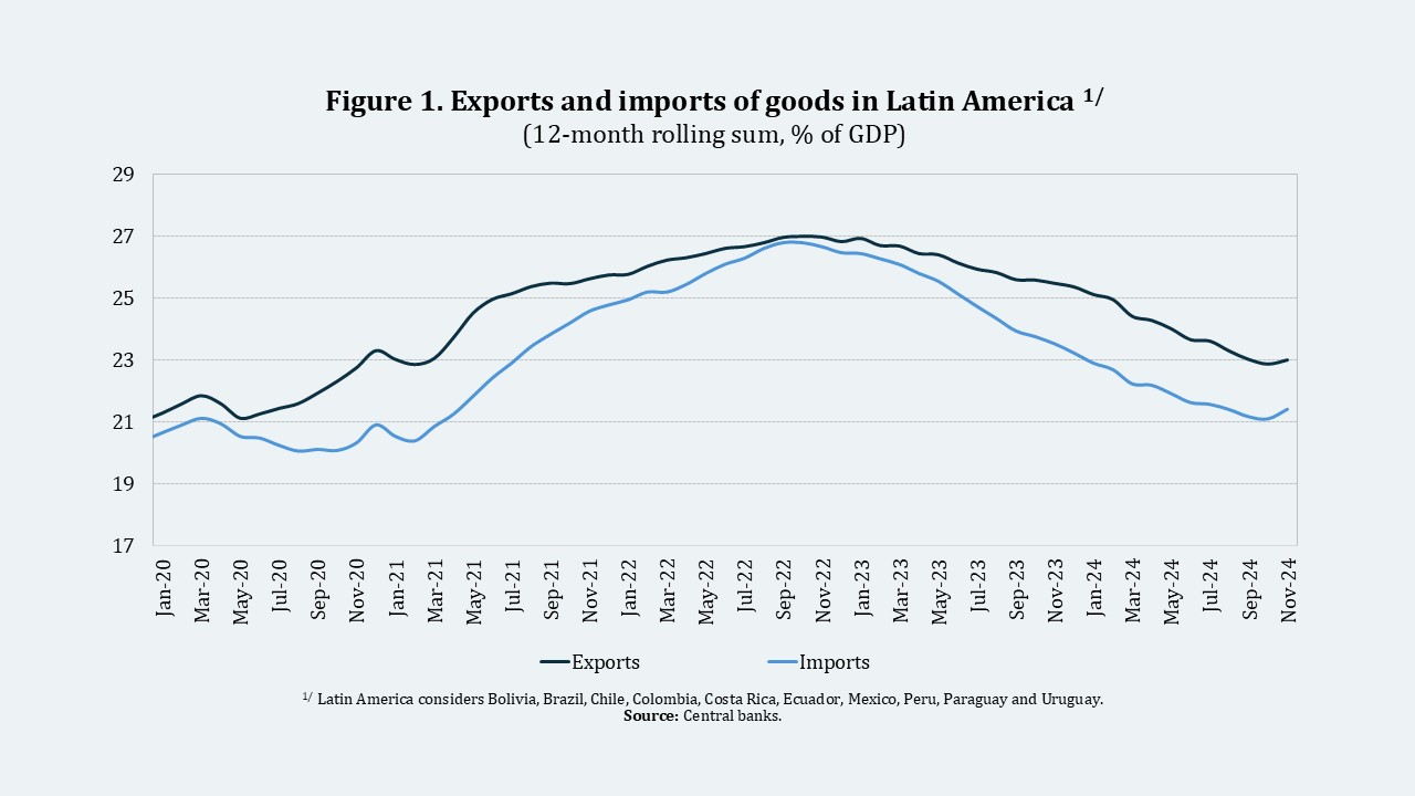
In 2024, the estimate of the region’s current account deficit in the balance of payments was slightly lower than in 20231. This was largely due to slower domestic demand, which led to a sharper drop in goods imports as a share of GDP compared to exports (Figure 1). At the same time, remittances remained a key component of external flows, averaging 3% of the region’s GDP in 2024.
Currencies across the region faced several episodes of volatility in 2024. To identify and measure these, we developed a multivariate factor stochastic volatility model that analyzes five regional currencies: Brazil, Chile, Colombia, Mexico, and Peru. Details of the model are provided in Box 1.
The most significant volatility episode occurred in early August (Figure 3), when global stock markets declined sharply, and there was a sudden sell-off of yen carry trade positions. This was triggered by the release of U.S. July labor market data, which raised recession fears amid a restrictive monetary policy environment. Simultaneously, the Bank of Japan increased its short-term interest rate after an extended period at historically low levels.
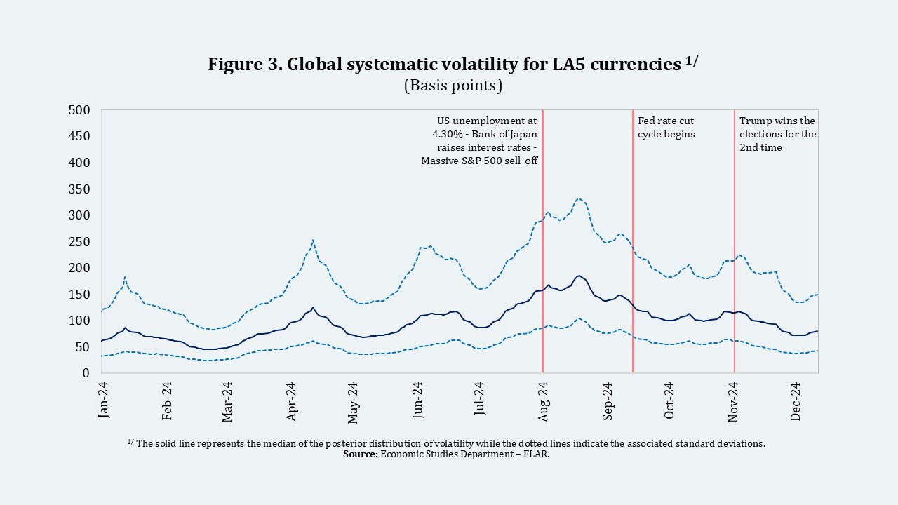
The start of the Federal Reserve’s rate-cutting cycle contributed to a reduction in currency fluctuations in the region. In contrast, the outcome of the U.S. elections caused moderate currency volatility in Latin America, though it was less pronounced than in 2016 (see Box 1).
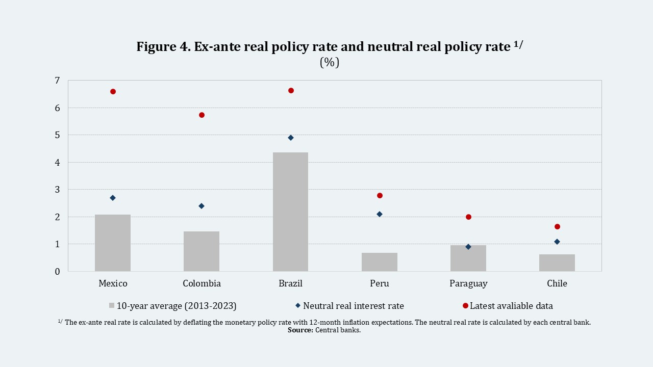
Inflation in the region continued to decline in most countries but remained above target levels, mainly due to the price of services. While short- and medium-term inflation expectations stayed relatively anchored, the latter saw an uptick in several countries, including Brazil and Chile. Against this backdrop, most central banks chose to pause their rate-cutting cycles, while Brazil’s central bank raised its rate four times. As a result, real interest rates remained in restrictive territory, staying above neutral levels (Figure 4).
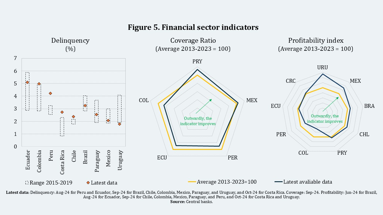
The financial system showed mixed performance but remained resilient. In several countries, credit growth slowed, delinquency rates remained high, and return-on-equity stayed low (Figure 5).
Latin America’s GDP is expected to slow further in 2025, with annual growth projected at 1.9%. This slowdown is driven by lower prices for key regional commodities and potentially weaker external demand amid ongoing geopolitical uncertainty. Prices for oil and soybeans, for example, are likely to come under pressure from positive supply shocks, such as the relaxation of OPEC+ production cuts. Additionally, potential new U.S. tariffs and a stronger dollar could pose headwinds for industrial metals.
Inflation in the region is expected to continue falling, averaging 3.5% by the end of 2025. Most countries are expected to reach their central banks’ target ranges or levels.
The baseline forecast scenario faces several risks. Trade policies from the new U.S. administration, such as additional tariffs and other restrictions, could create further uncertainty shocks, affecting trade, investment, and remittances to the region (Giraldo et al., 2023).
Additionally, a potential resurgence of inflationary pressures could prompt central banks to tighten monetary policy further. In this context, fiscal and macro-financial risks could intensify. Moreover, high levels of public debt, coupled with greater reliance on external debt in some countries, could amplify the effects of currency volatility triggered by global events (see Box 1).
In short, Latin America is heading into a challenging 2025, shaped by global headwinds and internal structural challenges. However, it also presents opportunities to reinforce and build on progress in macroeconomic stability.
1 The Economic Studies Department estimate suggests that the region’s current account deficit will decrease from 1% of GDP in 2023 to 0.9% of GDP.
Box 1. Exchange rate volatility in LATAM - Global Factor FX-LA5
Studies such as Forero (2022)1 show that exchange rate volatility in the region can be decomposed into two main factors: The first component is associated with systemic or common volatility, which arises from episodes of global uncertainty that affect currencies in a synchronized manner, albeit to different extents. The second component corresponds to the idiosyncratic volatility inherent to each currency, influenced by specific domestic factors.
Since these two underlying components of exchange rate volatility are not directly observable, the estimation follows the methodology proposed by Kastner, Frühwirth-Schnatter, and Lopes (2017)2, employing a Multivariate Factor Stochastic Volatility Model, using efficient Bayesian inference techniques.
The Model
Let \(y_{jt}\) be the logarithmic return for currency \(s_{j,t}\) of country \({j}\) of LATAM
\(
y_{jt} = \ln \left( \frac{s_{j,t}}{s_{j,t-1}} \right)
\)
\(
j = 1, \dots, m
\)
Let be the vector of the \(m\) exchange returns \(y_t = \left( y_{1t}, \dots, y_{mt} \right)’\) and the vector of the \(r\) unobservable global latent factors \(f_t = \left( f_{1t}, \dots, f_{rt} \right)’\). The vector of returns is assumed to be determined by these latent factors and idiosyncratic innovations..
We assume that the conditional log-variance of both idiosyncratic shocks \(h_t^u = \left( h_{1t}, \dots, h_{mt} \right)’\) as latent factors \(h_t^v = \left( h_{m+1,t}, \dots, h_{m+r,t} \right)’\) are variable over time. Therefore, there are \(m + r\) latent log-variances \(h_t = \left( h_t^u, h_t^v \right)\) in total.
- Conditional Mean Equation
\(y_t = \Lambda f_t + U_t \left( h_t^u \right)^{\frac{1}{2}} \varepsilon_t\)
\(\varepsilon_t \sim \text{iid } N\left( 0_m, I_m \right)\)
- Global Latent Factors Equation
\(f_t = V_t \left( h_t^v \right)^{\frac{1}{2}} \zeta_t\)
\(\zeta_t \sim \text{iid } N\left( 0_r, I_r \right)\)
Where \(\Lambda\) is a matrix of dimension \(m x r\) and represents the sensitivity (factor loadings) of exchange rate returns to global latent factors. On the other hand, the conditional variance and covariance matrices corresponding to the idiosyncratic shocks \(U_t(h_t^u)\) and the global latent factors \(V_t(h_t^v)\) are diagonal and of dimensions \(m x m\) and \(r x r\), respectively.
\(U_t(h_t^u) = (\exp(h_{1,t}), \cdots, \exp(h_{m,t}))\)
\(V_t(h_t^v) = (\exp(h_{m+1,t}), \cdots, \exp(h_{m+r,t}))\)
- Stochastic Log-Volatility Equation
All variances are in turn modeled as latent variables, whose logarithms follow independent autoregressive stochastic processes of order one.
\(h_{it} = \mu_i + \phi_i(h_{i,t-1} – \mu_i) + \sigma_i \eta_{it}\)
\(\eta_t \sim iid\ N(0_{m+r}, I_{m+r})\)
\(i = 1, \cdots, m+r\)
Where the parameter \(\mu_i\) represents the level, \(\phi_i\) captures the persistence, and \(\sigma_i\) (also known as Vol-Vol) measures the standard deviation of the log-variance.
- Breakdown of LATAM Exchange Rate Volatility
Finally, we can disaggregate the conditional variances of exchange rate returns as follows
\(\Sigma_t(y_t / h_t) = \Lambda V_t(h_t^v)\Lambda’ + U_t(h_t^u)\)
Since the matrices are diagonal, the exchange rate volatility of country \(j\) is determined by the sum of the volatilities of the \(r\) global latent factors common to the region, weighted according to the degree of exposure or sensitivity of its currency to these factors, and by the idiosyncratic volatility specific to the country.
The data used correspond to the daily exchange rate returns for the currencies of the region (Brazil, Chile, Colombia, Mexico and Peru) during the period from January 2016 to December 2024. To estimate the model, we consider 2 global latent factors in order to improve the identification process.
We identify the volatility of the first latent factor as that which comes from the financial uncertainty of developed economies, especially the United States, as evidenced by the correlation of 0,6 with the short-term volatility measured by the VIX index. It was also observed that the Mexican peso had the highest level of exposure to this first factor, consistent with the close commercial relations that this country maintains with the United States. On the other hand, the volatility of the second latent factor would be related to the prices of commodities, with the Chilean and Colombian pesos having the greatest exposure to this factor. Likewise, the Peruvian sol stands out as the currency with the lowest fluctuations compared to its regional peers. Being a partially dollarized economy, its Central Bank carries out foreign exchange intervention through purchases and sales of dollars in the spot and forward markets.
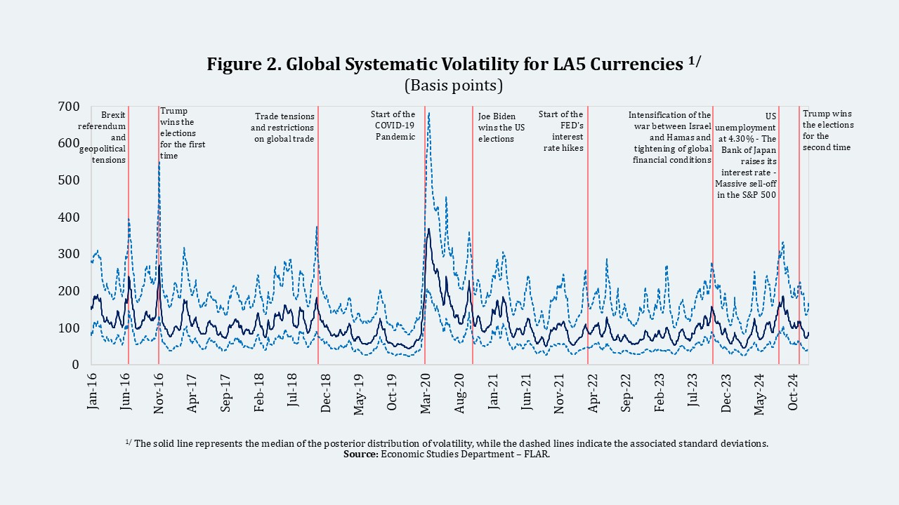
In general terms, the global volatility factor, which synchronizes the fluctuation of Latin American currencies, hereinafter referred to as the Global Factor FX-LA5 (GFX5-Index), captures historical episodes of global turbulence with depreciation effects on domestic currencies.
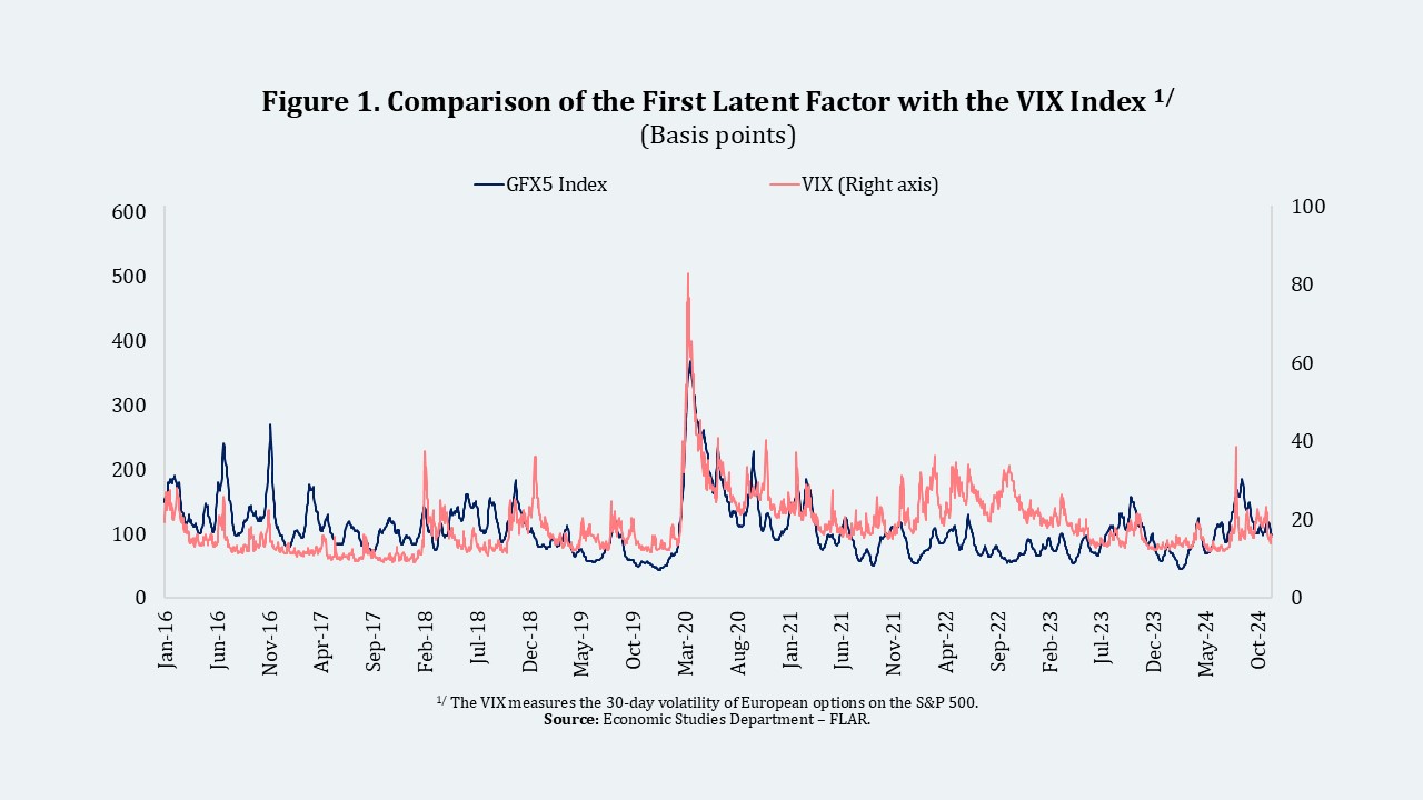
By November 2024, the sources of external volatility that have affected the region’s currencies following the U.S. presidential election reached 115 basis points, a more bounded level compared to 245 basis points in the 2016 election. In particular, the most relevant episodes recorded by the GFX5-Index in the last year are linked to the increase in the probability of recession in the United States, following the publication of weak employment data in July, in an environment characterized by a restrictive monetary policy. In addition, the increase in the short-term interest rate by the Bank of Japan, after a prolonged period at historically low levels, stands out. These events triggered sell-offs in global stock markets and a sudden deleveraging of yen carry trade positions in August 2024. Under this episode, global volatility contributed 183 basis points to regional currency volatility, a level not seen since the COVID-19 pandemic, surpassing even the 148 basis points recorded during the height of geopolitical tensions in the Middle East and the tightening of global financial conditions in October 2023.
1 Pérez Forero, F. J. (2022). Exchange rate volatility in LATAM: Common and idiosyncratic factors (Documento de Trabajo No. 2022-001). Banco Central de Reserva del Perú. https://www.bcrp.gob.pe/docs/Publicaciones/Documentos-de-Trabajo/2022/documento-de-trabajo-001-2022.pdf
2 Kastner, G., Frühwirth-Schnatter, S., & Lopes, H. F. (2017). Efficient Bayesian Inference for Multivariate Factor Stochastic Volatility Models. Journal of Computational and Figureical Statistics, 26(4), 905–917.